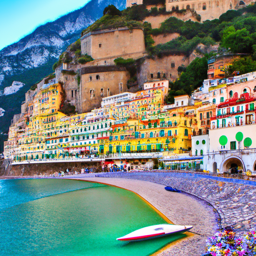
This project involved using a pre-trained diffusion model to produce many interesting images - for example, inpainting, hybrid images, and optical illusions.
After that, the second part of the project involved creating a diffusion model from scratch using a complex architecture of convolutional layers, max pooling layers, and other things, which was used to train on and randomly sample MNIST digits.
First, I tested the pre-trained diffusion model by generating a few images and varying the num_inferences parameter.
Shown below are selected results for a few values of num_inferences. Notice how as num_inferences increases, the quality of the images increases significantly.


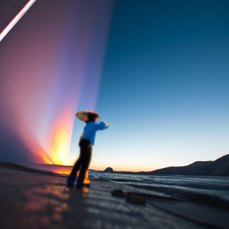
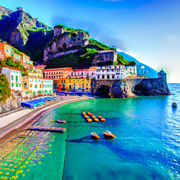
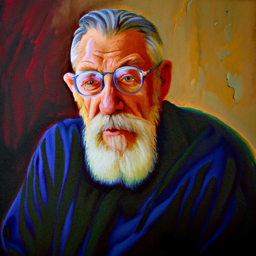
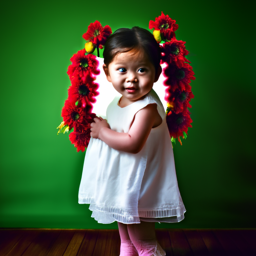
After testing out the pre-trained diffusion model, I implemented the forward process for adding appropriate noise to the image. Specifically, I did this by generating a random image using torch.randn_like, and adding this multiplied by a factor between 0 and 1 to the original image
Shown below are the results for no noise, t=250, t=500, and t=750 (the t values control the noise factor based on the pre-computed alphas_cumprod list)


After this, I implemented classical denoising using the torchvision.transforms.functional.gaussian_blur with a kernel size of 7 to blur the noise out of the image.
The results for this were not very good, especially for high levels of noise, and were meant more as a baseline for future, improved denoising techniques.


Next, I implemented one-step denoising by passing in the noisy image to the pre-trained UNet model. This model predicts the nosie in an image, and we can recover the original image by subtracting this noise estimate from the noisy image, subject to some multiplicative factors that depend on the pre-computed alphas_cumprod list.
The results for this, as seen below, were significantly better than that of classical denoising.


After doing One-Step Denoising, I improved this by performing iterative denoising. For a given value of t, I run the pre-trained UNet to get the current noise prediction. There are too many values of t for denoising every single step to be practical, so instead, I step through every 30 values of t, using an interpolation formula to compute the current image at every iteration, which will progressively get less noisy as t gets lower. Shown below are some intermediate results of denoising the Campanile using this method, starting with a noise value determined by t=690, as well as the final results compared to methods used earlier. Notice how much better iterative denoising is compared to the alternatives.


From here, to generate randomly sampled images, I simply perform the iterative denoising process from an image of pure noise. 5 results of calling this sample function are shown below:


To improve the sampling results, I added classifier-free guidance: by adding to the noise estimate an extra term of gamma * (noise - unconditional noise), where gamma=7 here and unconditional noise is the noise calculated by running the UNet on an empty prompt. This improved the results, as seen below for another 5 random samples:


Using this sampling algorithm, we can generate sample images that progressively look more and more similar to the test image, by starting at values of t other than pure noise. Shown below is this process applied to three images: the Campanile; a photo of my family's cat, Miso; and a photo of myself. From left to right, notice how the images gradually get more and more similar to each test image.


This process works well when applied to hand-drawn images, in addition to just regular images. Shown below is the same process applied to three new images: an illustration from the web of Mt. Rainier, and crude drawings I made of a tree and of a diver, respectively.


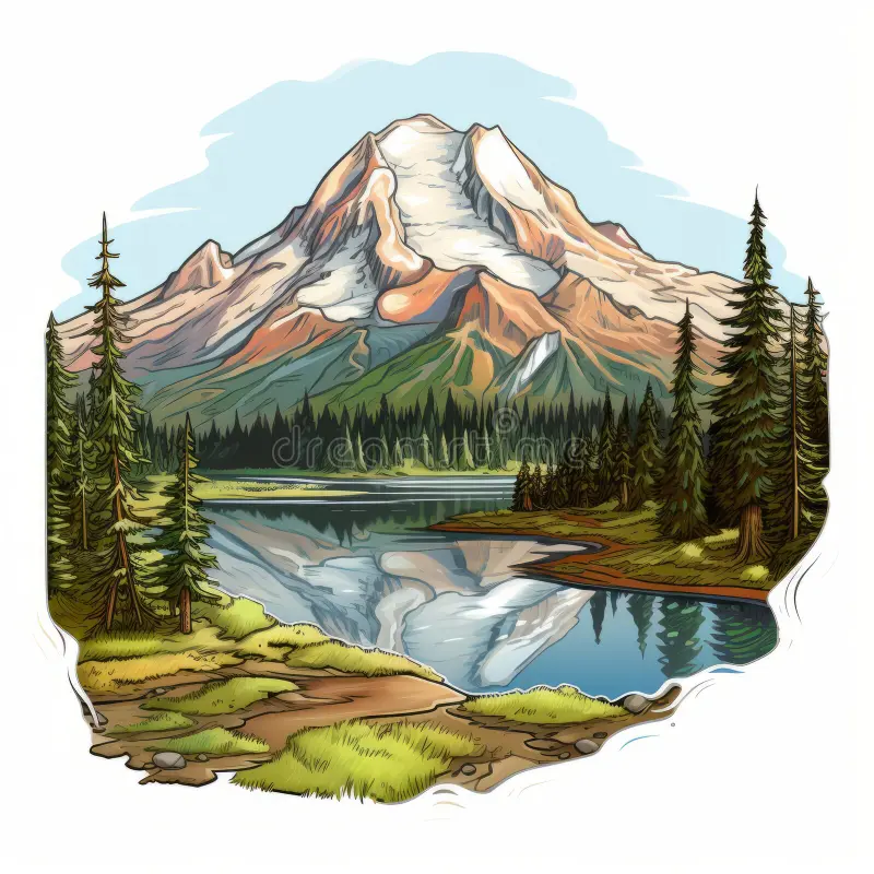


We can also apply this technique to inpainting images - where we take a test image, create a mask, blur out the mask from the test image, and denoise the image separately for the masked section and the rest of the image, producing a guess as to what the masked portion originally contained. I tried this on the Campanile image (masking the tip of the tower), the image of Miso (masking his head), and the image of myself (masking my head), with results shown below:


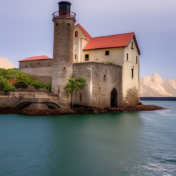
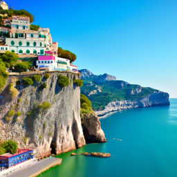
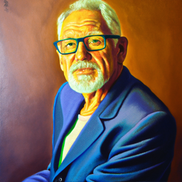
As one last modification to the CFG algorithm from 1.6: we can apply a similar technique to 1.7, where we sample images with different i_start values; however, this time, I used other prompts than "a high quality photo". That way, an image will start out looking like the prompt, and gradually become more similar to the test image. Specifically, I first tried "a photo of the amalfi coast" as the prompt and the Campanile as the test image. Next, I tried "an oil painting of an old man" and the photo of myself, producing some funny results near the end. Finally, I tried "a photo of the amalfi coast" once again as the prompt, this time using a photo I took of the Salmon River Reservoir as the test image.


Next, I applied the methods of the CFG sampling algorithm to solve a more difficult problem: sampling visual anagrams; specifically, generating an image that looked like one prompt right side up, and another prompt upside down.
I accomplished this by generating two noise estimates: one for the regular image with the first prompt, and the other of the flipped image with the second prompt, flipping the result of the latter noise estimate. Doing this for both the conditional and unconditional noise estimates and averaging each of the results for the two prompts together, I proceed with the CFG algorithm as normal, performing this modified process on every iteration.
I tried this on three image pairs, having to try a lot of different samples for each before finding a reasonable result. First, I reproduced the assignment image of an old man and people around a campfire. Then, I made an image that looked like Mt. Rainier when looked at right side up, and looked like a huge ship when looked at upside down. Finally, I made an image that also looked like Mt. Rainier when shown right side up, but looked like a bowl of pasta when shown upside-down. Results are shown below:


For the final task of Part A, I used a similar technique to the previous section to generate hybrid images: images that looked like one thing close up, and another thing far away.
I accomplished this in a similar manner to the visual anagrams, except that I didn't flip the images this time, and instead of just averaging the noise values, I applied a low-pass filter to one, and a high-pass filter to the other.
I applied this to three image pairs: a hybrid image of a skull and a waterfall like the example from the project description, a hybrid image of Mt. Rainier and a rocket ship, and finally, a hybrid imgae of a man wearing a hat and a rocket ship.


After using the pre-trained DeepFloyd model in Part A, in Part B, I set out to train my own UNet and use this to sample MNIST digits.
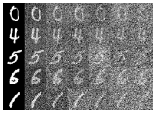
I started by applying noise to MNIST digits with varying levels, as shown in the first image.
Then, I used various torch.nn modules to construct a full UNet for single-step denoising, training this UNet on MNIST data with partial (0.5) noise applied to them.
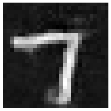
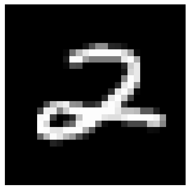
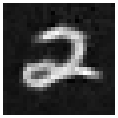
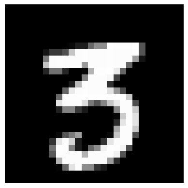
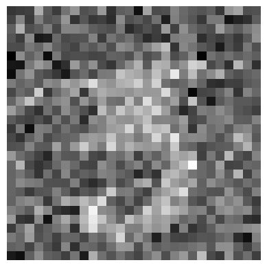
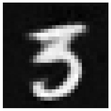
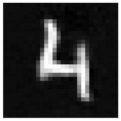
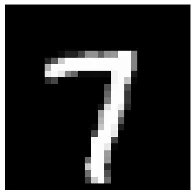
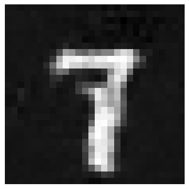
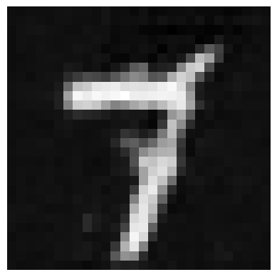
After training for 5 epochs using the L2 loss between the predicted image and the real image, my model achieved reasonably low loss, and successfully recovered the original, noiseless digits for several examples shown below.
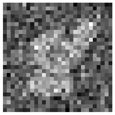
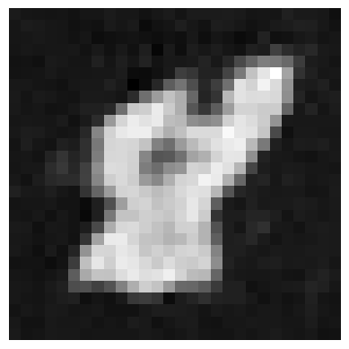
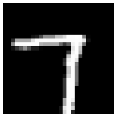
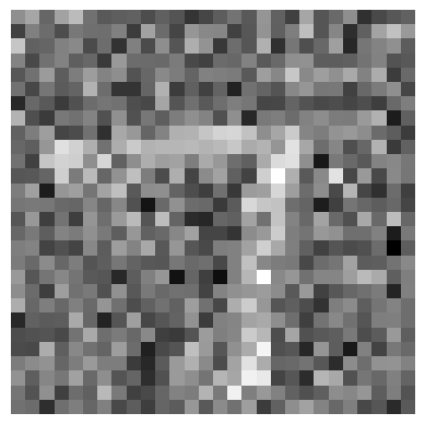
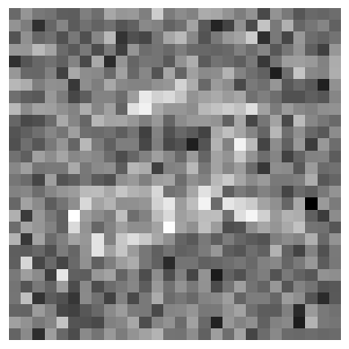
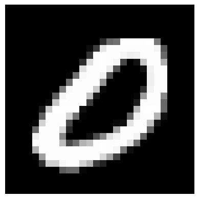
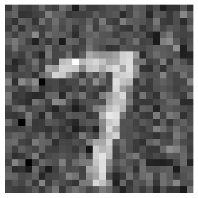
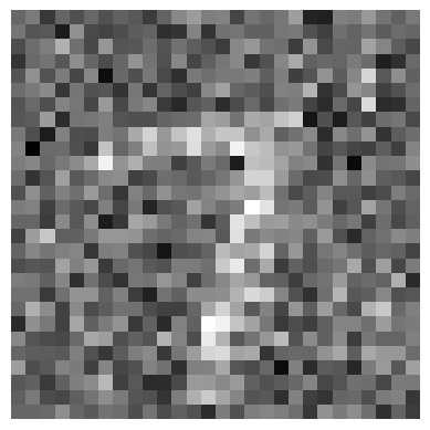
Lastly, I tried denoising images with different noise values (i.e. not just 0.5) using my UNet, with varying results, also shown below.

After successfully training a single-step denoising model, I proceeded to train a time-conditioned model to be able to produce sample MNIST digits from completely random noise.
I accomplished this by adding two FCBlock network layers to the model, each of which takes in t as a parameter. I also modified the training of the algorithm to predict the noise added instead of the original image.
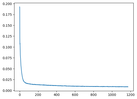
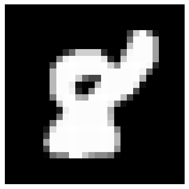
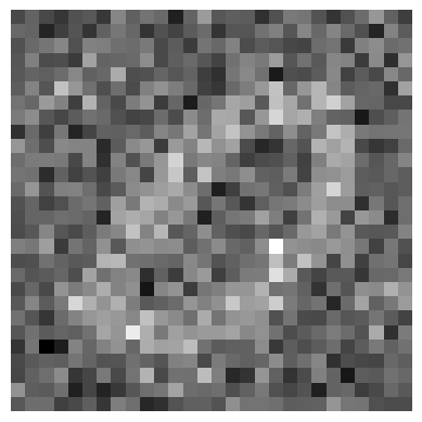
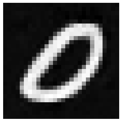
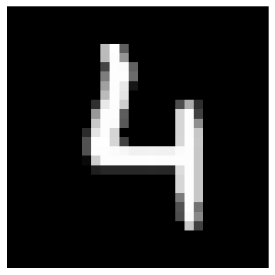
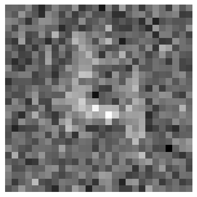
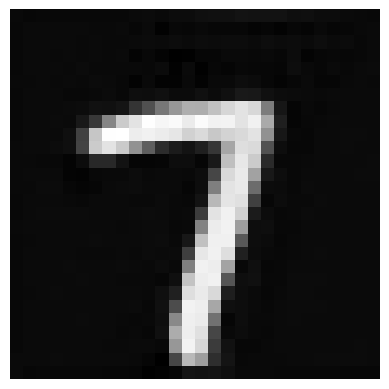
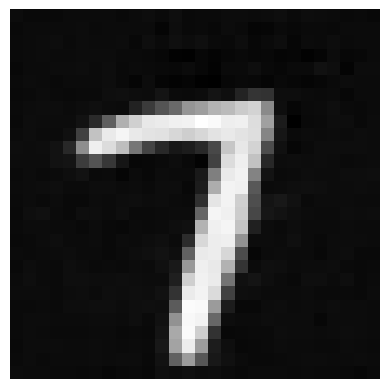
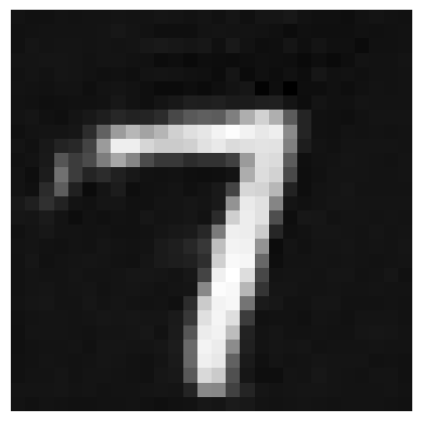
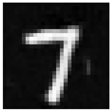
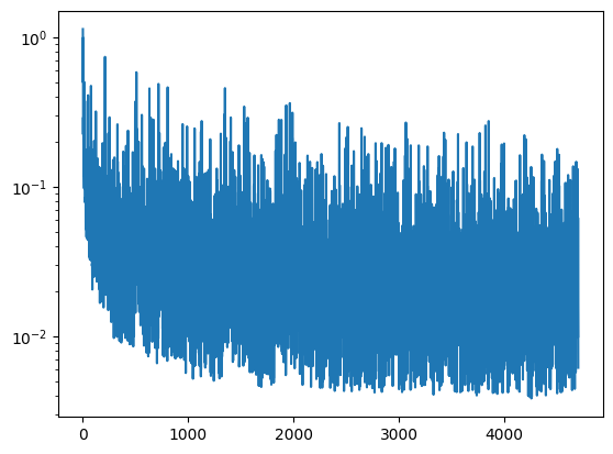
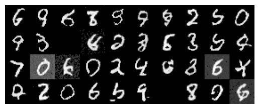
After this, I ran a similar algorithm to my algorithm from part A1.4 with the pre-trained UNet, generating random MNIST digits. Although the loss curve jumped around a bit, the actual image results, shown below for epochs 5 and 20, were promising.
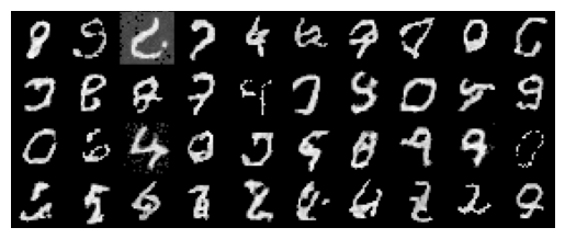
Finally, I added class condition to the model from earlier, in order to generate random samples of specific digits. I did this by adding an additional parameter, c, to the forward function - a one-hot encoding of the digit to generate a sample of. I conditioned the model based on this parameter by multiplying two of the intermediate values by this c parameter, in the same place where I add the FCBlock applied to t.
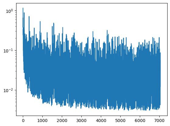
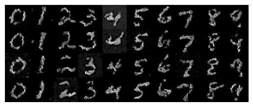
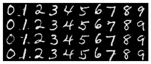
This once again produced a somewhat funky loss curve, but the results looked good for every digit - shown below for epochs 5 and 30.
Overall this was a very interesting project and I had a lot of fun both playing around with pre-trained diffusion models, and training my own diffusion models. The biggest thing I learned from this project was to try running a sample multiple times if the first time didn't quite look right; especially, for parts A1.8 and A1.9 where the model was not specifically trained for the task at hand.